Translation Notice
This article was machine-translated by Gemini 2.5 Pro.
- Original Version: Authored in Chinese by myself
- Accuracy Advisory: Potential discrepancies may exist between translations
- Precedence: The Chinese text shall prevail in case of ambiguity
- Feedback: Technical suggestions regarding translation quality are welcomed
Preface
As the title suggests, this is an exploratory project of mine. Its purpose is not to achieve any specific result, but to learn through the process of experimentation. This article includes a brief technical report, as well as some insights and experiences gained along the way. The comment system is not yet set up, so if you have any thoughts or questions, please feel free to post them directly in the project’s Issues / Discussions.
Recently, I’ve been studying Reinforcement Learning (RL), and I’m particularly fond of the AlphaZero algorithm. It’s a general reinforcement learning algorithm that evolved from AlphaGo, which defeated world Go champion Lee Sedol in 2016. Some mainstream introductory books on reinforcement learning typically stop at methods like PPO, SAC, or DDPG (without covering the AlphaZero, MuZero series), which I personally believe is a significant omission.
Fundamentally, AlphaZero belongs to the category of Model-Based RL, which is inherently different from Model-Free RL represented by Q-learning and Actor-Critic. The key difference is its use of an environment model (a game simulator) to deduce the optimal policy through tree search, rather than gradually improving expected returns through extensive trial and error. A good environment model is crucial for the success of such algorithms; in board games, clear rules directly provide a perfect environment model. In contrast, the real physical world is incredibly complex and difficult to describe with simple rules, which has become a key bottleneck hindering the practical application of reinforcement learning. Meta’s recently open-sourced V-JEPA 2 is an important step towards building world models, and I highly recommend looking into it.
Due to limited computational resources, I chose Saiblo Connect Four as the game environment 1. Its state space is relatively small, yet it has a certain level of complexity with no known winning strategy. Additionally, the platform features excellent traditional methods for comparison, allowing for a relatively objective assessment of the algorithm’s playing strength. I am very grateful to Tsinghua University for providing this platform, which not only meets the experimental needs of its students but also offers great convenience to enthusiasts outside the university.
Since my AI uses some algorithmic improvements from KataGo, I named it katac4. The code is fully open-source on GitHub.
As of the time of writing (2025.06.27), katac4 is firmly in first place on the game’s ladder with a commanding lead:
![]()
A Quick Look at AlphaZero
There are many easy-to-understand articles about AlphaZero online, so I will only provide a brief, more abstract overview here (with ideas referenced from the KataGo paper).
The algorithm generates training data through self-play guided by Monte Carlo Tree Search (MCTS). The search process involves repeatedly expanding the game tree: each time, starting from the root node, a path is followed to a leaf node. At node $n$, the child node $c$ that maximizes the following formula is chosen for the visit:
$$ \mathrm{PUCT}(c)=V(c)+c_\mathrm{PUCT}P(c) \frac{\sqrt{\sum_{c'}N(c')}}{1+N(c)} $$Here, $V(c)$ is the average predicted utility value of all nodes in the subtree of $c$, $P(c)$ is the prior probability for the action corresponding to $c$ given by the neural network, $N(c)$ is the number of simulations previously run through node $c$, and the constant $c_\mathrm{PUCT}=1.1$; $c'$ represents all child nodes of $n$.
Unlike the $\epsilon$-greedy algorithm, AlphaZero enhances exploration by applying Dirichlet noise to the prior probabilities at the root node:
$$ P(c)=0.75P_{\text{raw}}(c)+0.25\eta $$where $\eta$ is sampled from a Dirichlet distribution with parameter $\alpha=0.8$, and $P_{\text{raw}}$ represents the raw policy distribution given by the neural network.
Let the root of the search tree have $k$ child nodes $u_1,\dots,u_k$, corresponding to actions $a_1,\dots,a_k$. Then the visit distribution of MCTS is proportional to $N(u_i)$:
$$ \pi(a_k|s_t)=\frac{N(u_k)}{\sum_{i=1}^k N(u_i)} $$This is the training target for the neural network and is also used to select the next move during self-play (sampled with a dynamically changing temperature $T$). Self-play starts from the initial board position. During inference (actual matches), the action with the highest probability in this distribution, i.e., the most visited one, is typically chosen directly.
The neural network takes the current board state $s_t$ as input and predicts the probability distribution of the next move $\pi$ and the win rate of the position $z$. Its loss function is:
$$ L=-c_g \sum_r z(r) \log(\hat z(r))-\sum_m \pi(m) \log(\hat \pi(m))+c_{L2} ||\boldsymbol\theta||^2 $$where $r \in \{\text{win}, \text{loss}, \text{draw}\}$ represents the game outcome from the current player’s perspective, and the constants are $c_g=1.5, c_{L2}=3\times 10^{-5}$. The entire loss function is a weighted sum of the following three parts:
- Cross Entropy between the win rate prediction and the actual result 2;
- Soft Cross Entropy between the policy distribution prediction and the MCTS visit distribution;
- L2 regularization on the neural network parameters $\boldsymbol\theta$.
Policy updates are done in an Off-policy manner, maintaining a replay buffer. After each self-play game is completed, the new experience data is added to the replay buffer, from which a mini-batch of size $B$ is sampled for gradient descent updates. The SGD with Momentum optimizer is used, with the learning rate adjusted according to the training phase.
Overall, AlphaZero is consistent with the core idea of policy iteration algorithms, but it uses MCTS to perform both policy evaluation and policy improvement tasks simultaneously.
Training, Annealing
The concept of annealing is crucial for successfully training an AlphaZero agent. This involves many details, and I recommend referring to the code. Here, I list a few key points:
- The temperature for sampling actions from the visit distribution is $T=0.8^{1+step/boardsize}$. AlphaZero_Gomoku uses a constant $T=1$, which in practice proves to be completely wrong. In the late game, “one false move can lose the whole game.” Directly sampling actions based on the visit distribution would generate a large number of incorrect game outcome samples, causing the entire training to collapse.
- For the policy given by the neural network, apply a temperature $T=\max(1.03,1.35\times0.66^{step/boardsize})$ at the root node. This ensures a certain level of exploration and enhances training stability.
- Learning rate annealing. For the early stage of training ($5\%$ of iterations), use $1/3$ of the normal learning rate (to prevent large fluctuations). After $72\%$ of iterations, use $1/10$ of the normal learning rate (to maximize playing strength improvement).
Many of these hyperparameters are not necessarily optimal and were set somewhat arbitrarily, but their combination has proven effective. I hope they can provide some reference value.
Algorithm Optimizations
Recomputing the AlphaGo Zero weights will take about 1700 years on commodity hardware.
This sentence is from the Leela Zero project’s README. AlphaZero’s exploration process is inherently inefficient, but well-designed algorithmic optimizations can significantly shorten its training cycle. The methods in the KataGo paper, when used together, can improve training efficiency by ~50x. Below are some of the optimizations I used, some of which are from KataGo.
Gradient Accumulation
Our game environment, Saiblo Connect Four, has variable board sizes, with both width and height ranging in $[9,12]$. This results in a total of $16$ different board sizes.
To adapt to different board sizes, two improvements were made:
- The neural network uses a fully convolutional (FCN) architecture 3, with the policy head’s output size matching the input state size.
- When sampling from the replay buffer, instead of directly sampling $256$ examples, we sample $16$ examples for each board size. We perform a forward pass for the samples of each board size, calculate the gradients, and accumulate them. Then, a normal backward + step is performed.
KataGo uses board masking to adapt to different inputs, which involves tedious implementation details. I chose the simpler approach of gradient accumulation, which, although slightly less efficient, is much more convenient.
Action Space Pruning
The motivation for this method is very simple: manually filter out moves that can be proven to be strictly wrong, treating them as illegal moves and excluding them from MCTS calculations.
The implementation requires very minor code changes and can be summarized by two rules:
- If I can win in one move, I must make that move;
- If the opponent can win in their next move, I must block it.
This optimization is very simple yet significantly speeds up exploration in the early stages of training, allowing the model to quickly understand the game’s rules. It also helps avoid some bad blind spots, especially when an opponent forms a threat of three near the edge of the board, which a CNN might overlook.
First Play Urgency (FPU)
This optimization originates from Leela Zero.
A careful reader might ask: when calculating PUCT, if a child node has not been visited, i.e., $N(c)=0$, how is $V(c)$ defined?
AlphaGo Zero provides the standard answer: $V(c)=0$. However, the Leela Zero community found that this is not the optimal choice. They chose:
$$ V(c)=V(n)-c_\text{FPU}\sqrt{P_\text{explored}} $$where $n$ is the parent node, the constant $c_\text{FPU}=0.2$, and $P_\text{explored}$ is the sum of the prior probabilities of all child nodes that have been visited at least once:
$$ P_\text{explored}=\sum_{c'|N(c')>0} P(c') $$Readers can ponder the rationale behind this approach. A discussion on Lc0’s GitHub points out that for a strong neural network, this method can lead to an improvement of ~200 Elo.
Playout Cap Randomization
Corresponds to Playout Cap Randomization in the KataGo paper.
The two output heads in AlphaZero require different numbers of playouts for optimal training. Some informal studies suggest that the most efficient number of simulations for training the policy head is very close to AlphaZero’s $N=800$, but in the first version of AlphaGo, even $N=1$ was sufficient to train a decent value head. To alleviate the tension between the two, we choose a smaller number of simulations $n < N$ and perform a fast search ($n$ simulations) with probability $p$, and a normal full search ($N$ simulations) otherwise. Samples generated from fast searches are not used for policy training4.
My hyperparameter choices are $(N,n)=(800,160)$ and $p=0.25$. I personally feel that for a game like Connect Four, the number of simulations could probably be even smaller.
Forced Playouts & Policy Target Pruning
Corresponds to Forced Playouts and Policy Target Pruning in the KataGo paper.
As mentioned earlier, AlphaZero introduces Dirichlet noise at the root node to enhance exploration. However, this method does not guarantee that good moves will definitely be discovered.
Imagine the following scenario:
- Game state $s_t$. The current neural network strongly favors move $a$, while the actual optimal move is $a^*$. In the output policy distribution, $a$ gets over $80\%$ probability, while $a^*$ gets less than $5\%$.
- Dirichlet noise is introduced. The probability of $a$ is still very high, while $a^*$ is “selected” and rises to $10\%$. Let’s assume $P(a)$ is now exactly $80\%$.
- MCTS visits $a$ and $a^*$ in sequence. The value network still doesn’t favor the state $s^*$ reached by $a^*$, preferring the state $s$ from move $a$, giving $V(s^*)=-0.8$ and $V(s)=-0.1$.
- The total number of simulations is now $N=2$. According to the PUCT formula, we have $\text{PUCT}(a)=0.34$ and $\text{PUCT}(a^*)=-0.745$. The PUCT values are already vastly different. If MCTS continuously selects $a$ for visits and $V(s)$ remains unchanged, it would take nearly $200$ simulations before $\text{PUCT}(a^*)\ge\text{PUCT}(a)$. By then, $1/4$ of the simulations have been wasted. And if $a^*$ is given a poor evaluation again, it would take a long time to get another visit.
This shows that even if Dirichlet noise luckily falls on the correct move, the combined blind spots of the policy and value networks may still not be handled correctly. Therefore, we introduce a Forced Playouts mechanism to ensure that each child of the root node receives at least $\lceil n_\text{forced} \rceil$ visits:
$$ n_\text{forced}(c)=\left(kP(c)\sum_{c'}N(c')\right)^{1/2} $$
Following KataGo’s setting, the constant is $k=2$.
At the same time, to eliminate the significant noise introduced by both Dirichlet noise and Forced Playouts, we perform policy target pruning on the visit distribution after MCTS is complete:
- Find the child $c^*$ with the most visits $N(c)$.
- For other child nodes $c$, subtract as many visits as possible, ensuring that $\text{PUCT}(a^*) > \text{PUCT}(a)$ and that the number of subtracted visits does not exceed $n_\text{forced}(c)$.
I chose to directly solve the inequality to find the pruned visit count:
$$ N'(c)=\mathrm{clip}\left(\left\lceil\frac{P\sqrt N}{V+\text{PUCT}(c^*)}-1\right\rceil,N-n_\text{forced},N\right) $$For readability, the formula above uses $N$ for $N(c)$, $P$ for $P(c)$, etc.
Below is a comparison of the effect with/without policy pruning from the KataGo paper. Black: $p \approx 2\times 10^{-4}$; Green: $p \approx 1$.
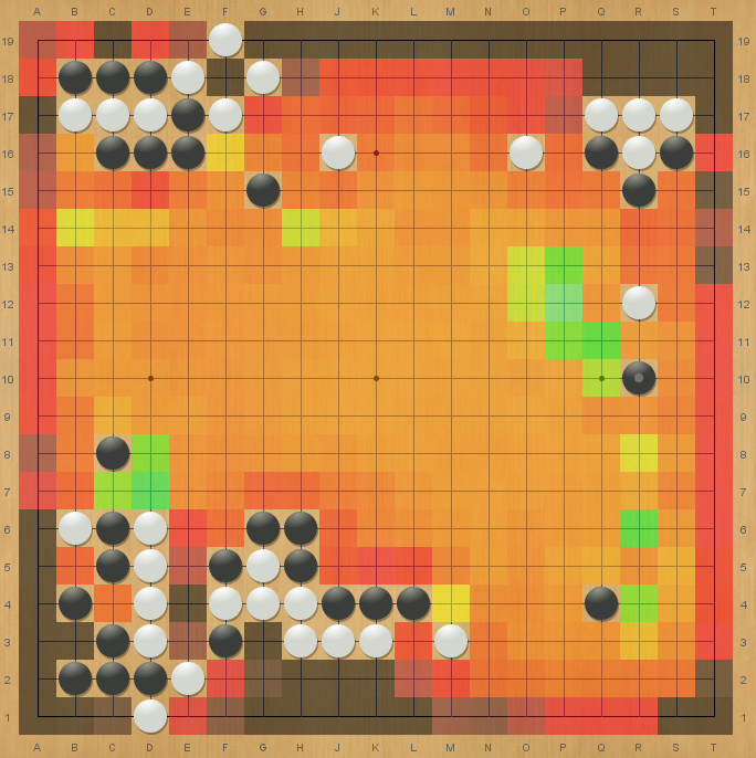 |
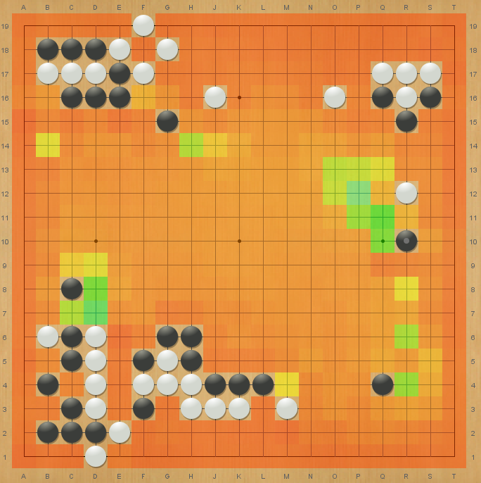 |
|---|---|
| With Policy Pruning | Without Policy Pruning |
Dynamic Replay Buffer
From Appendix C: Training Details in the KataGo paper.
In off-policy reinforcement learning algorithms, the size of the replay buffer (number of samples it can hold) is mostly fixed, often set in the range of $[2^{14},2^{20}]$. We, however, adopt a sub-linear growth strategy:
$$ N_{\text{window}} = c \left( 1 + \beta \frac{ ( N_{\text{total}} / c ) ^ \alpha - 1} { \alpha } \right) $$where $N_{\text{total}}$ is the total number of samples generated so far in the training process, and $c=250000, \alpha=0.75, \beta=0.4$. This is essentially applying a linear transformation to $f(n)=n^\alpha$ such that $f(c)=c$ and $f'(c)=\beta$. This allows for the rapid discarding of low-quality moves generated in the early stages and increases the diversity of training samples later on, effectively suppressing overfitting.
Monte Carlo Graph Search (MCGS)
See KataGo/docs/GraphSearch.md. Many thanks to David Wu for the easy-to-understand explanation; during this project, I even found a typo in it and fixed it with a PR 😆
The overall idea:
-
Implement Zobrist hashing for board positions. When expanding leaves, prioritize looking up identical state nodes in a hash table, turning the search tree into a DAG;
-
Calculate PUCT based on the visit counts of action edges (not nodes);
-
Use incremental updates during backpropagation:
$$ V(n) \larr \frac{1}{N(n)} \left(U(n)+\sum_c N(c)V(c)\right) $$Note that $U(n)$, the utility estimate from the value network, is essential.
In practice, memory management for MCGS can be tricky. Fortunately, the search trees generated by AlphaZero are not very large, so I just do a DFS cleanup. Currently, MCTS is still used for training, while MCGS is used for inference.
Engineering Optimizations
Since the project code is 100% Python, achieving full resource utilization is nearly impossible. However, there are still some tricks to improve training efficiency.
Parallel Self-Play
This idea is easy to understand and can be applied to most mainstream reinforcement learning algorithms. Use multiple processes in parallel on different GPUs to collect training data and send the results to a main process for model updates.
Currently, I use a total of 20 different processes for self-play, distributed evenly across 4 GPUs. Note that you should use torch.multiprocessing instead of Python’s built-in multiprocessing module.
CUDA Graphs
This is another relatively general optimization technique that can be used in many machine learning applications. The principle is to send the entire computation graph to the GPU for execution, significantly reducing front-end/back-end interaction and kernel launch overhead 5. For smaller networks and batch sizes, CUDA Graphs can provide an unexpected speed boost.
The project’s root directory provides a (rudimentary) benchmark script. The results on a single RTX 4090 are as follows (batch_size=1 to simulate the self-play environment):
| Category | Inference Method | Computation Speed (FPS) |
|---|---|---|
| Base | torch.no_grad |
$249.1$ |
| Base | torch.inference_mode |
$265.9$ |
| TorchScript | torch.jit.script |
$271.5$ |
| TorchScript | torch.jit.trace |
$501.4$ |
| CUDA Graphs | torch.cuda.graph |
$3184.5$ |
Additionally, torch.compile(mode='reduce-overhead') can also achieve CUDA Graph-based inference. However, this API is not supported on Windows and has a compilation-time cost, making it less convenient than torch.cuda.graph.
Test Results
Training lasted for about 14 days, totaling $30000 \times 16$ iterations. First, here are the curves for Loss, Entropy (policy entropy), and episode_len (self-play game length) during training:
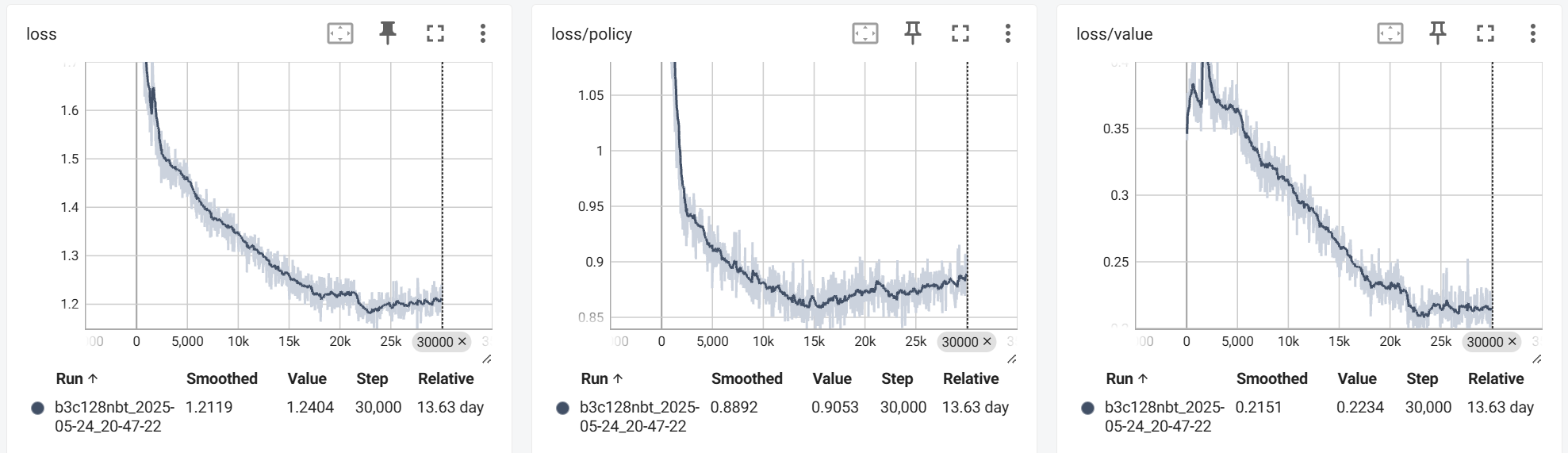
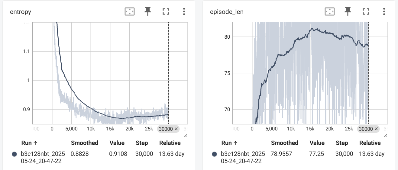
The loss and entropy decrease rapidly at the beginning and then stabilize (they don’t converge to $0$ because the data distribution is constantly changing); episode_len increases initially and then slightly decreases (possibly due to finding faster winning lines). Overall, this is in line with intuition and shows no unexpected behavior.
Next is the Elo6 rating curve, reflecting the actual playing strength:
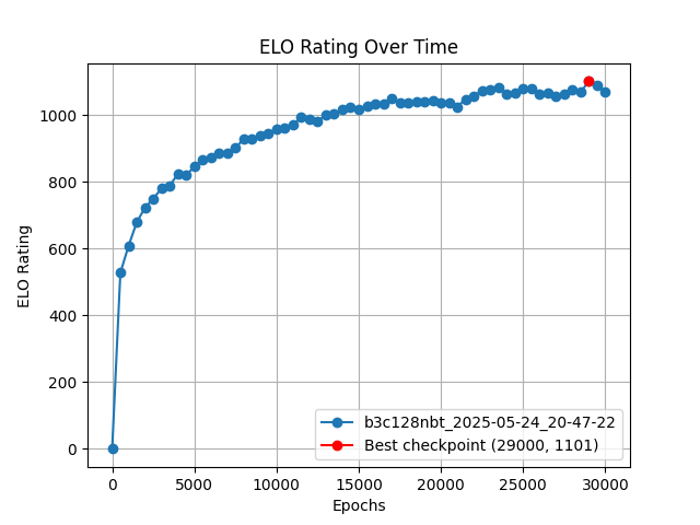
Overall, the training process was very stable (approximately sub-linear growth), and the training eventually reached near-saturation.
The best traditional method for the same task, under the same computational power, has only about a 26% win rate against katac4’s best checkpoint, corresponding to a -182 Elo difference. As seen in the graph, we reached a comparable level with just 1/4 of the iterations (3 days of training).
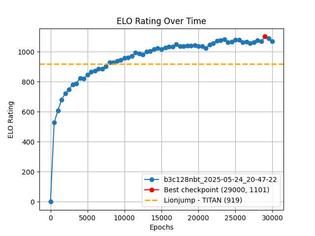
In reality, this estimate is not precise—the Epoch 6500 checkpoint can also achieve a win rate of over 50% against it. The above graph is for reference only.
I am very grateful to this predecessor for recently open-sourcing his method; in the early stages of my project’s development, I was always curious how he managed to lead the leaderboard by such a margin. A few days ago, I read his project report and was surprised to learn that even traditional methods perform better with PUCT than with UCT. To be honest, if I weren’t allowed to use a neural network, I probably wouldn’t even make it to the first page of the overall rankings.
Here are the test results against the Saiblo platform’s sample AIs:
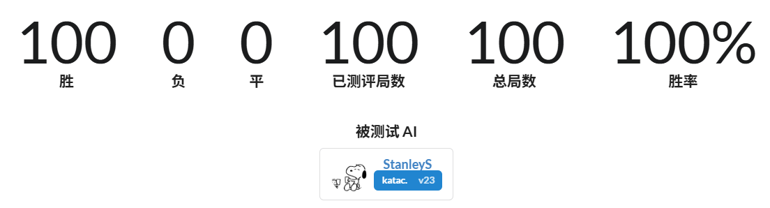
This result sometimes fails to run due to TLE. The strongest checkpoint has never lost (tested for $6\times100$ games), except for TLEs. The platform only has CPUs, so the inference solution uses TorchScript. However, import torch and torch.jit.load both have time overhead. When the evaluation server is under heavy load, it might TLE before the model even finishes loading. There’s really nothing I can do about this. (Sigh)
A few suggestions for the platform:
- Support LibTorch, so I can write inference in C++ and eliminate the import time;
- Provide some lightweight inference frameworks (like ONNX Runtime) to also alleviate slow loading issues.
- As a fallback, the time limit for the first move could be relaxed a bit…
I also created a for-fun version called fastc4, which directly selects the move with the highest probability from the neural network’s output. This version is actually not bad either:
- 97% win rate against the sample AIs;
- 65% win rate against jiegec/FourChess;
- 48% win rate against frvdec (former rank 2);
- 45% win rate against Lionjump0723/connect4 (former rank 1).
After manually observing some games, I feel that the neural network cares more about long-term gains—it plans for many moves ahead and doesn’t care about local gains or losses. Traditional methods are naturally focused on short-term tactical calculations and appear much weaker when there is no obvious winning sequence. My AI often loses to other AIs in the first 25 moves due to a tactical blind spot, but by move 50, the position is almost completely under its control. The traditional algorithms are powerless in the late game due to early strategic mistakes. This is somewhat similar to the difference between Stockfish and Leela Chess Zero in chess engines—the former is a meticulous calculator, while the latter relies more on intuition.
I hope these insights can help with the future development of traditional AI methods. I also welcome everyone to play against and test katac4 on the platform:
- katac4 (Epoch 29000):
96c96ac2389547958141d932d9279efc - katac4 (Epoch 30000):
2c9bd80e1e0e480a8f32214448880a62 - katac4 (Epoch 6500):
d4e85acaf1ab4025b3c6a7ebec4fd0f0 - fastc4 (Epoch 29000):
941dafdce03640bfb7ceb3aa32613252
Future Improvement Directions
There are currently two main issues:
- Low hardware utilization efficiency;
- Many early-game blind spots in the model.
In the future, I will consider merging leaf states from different self-play games into one large batch, which should largely solve the first problem.
For the second problem, besides increasing the model size (the next model is planned to be b5c128nbt), there are some algorithmic optimizations yet to be implemented:
- Add auxiliary policy heads (opponent’s next move distribution, game’s final move location, soft policy) to aid training;
- Optimize the board state representation (positions of moves from more previous turns, positions of threats of two or three, etc.);
- Discard fast game policy samples from Playout Cap Randomization;
- Use importance sampling proportional to $D_\mathrm{KL}(\hat{\boldsymbol\pi}||\boldsymbol\pi)$ to focus training on incorrectly predicted positions;
- Replace Batch Norm with Batch Renorm to prevent inconsistencies between the model’s training and inference behavior.
I’ll try to implement some of these if I have time this summer. Anyone who is interested is also welcome to contribute PRs with improvements. You are always welcome!
Further Reading
- Mastering the game of Go without human knowledge
- Mastering Chess and Shogi by Self-Play with a General Reinforcement Learning Algorithm
- Accelerating Self-Play Learning in Go
- Other Methods Implemented in KataGo
- Sayuri Go Engine Development Log
-
Game rules can be found in the documentation. ↩︎
-
The original AlphaZero directly predicts the position value $V(s_t) \in [-1,1]$ and uses MSE Loss. Here, I adopted the improved approach from KataGo and Leela Zero. ↩︎
-
The neural network design also references KataGo, using Global Pooling and Nested Bottleneck Residual Nets. The current version is named
b3c128nbt, indicating 3 nested bottleneck residual blocks with 128 channels. For brevity, I won’t detail the model design optimizations here; interested readers can refer to the code. ↩︎ -
My code implementation does not do this, and it doesn’t seem to have a major impact. However, removing them would likely be a better choice, and I plan to test this later. ↩︎